Mapping Many Gene Expression Traits
Overview
Teaching: 30 min
Exercises: 30 minQuestions
How do I map many genes?
Objectives
To map several genes at the same time
Load Libraries
library(tidyverse)
library(knitr)
library(broom)
library(qtl2)
library(qtl2ggplot)
library(RColorBrewer)

source("../code/gg_transcriptome_map.R")
source("../code/qtl_heatmap.R")
Before we begin this lesson, we need to create another directory called results in our main directory. You can do this by clicking on the “Files” tab and navigate into the main directory. Then select “New Folder” and name it “results”.
Load Data
# expression data
load("../data/attie_DO500_expr.datasets.RData")

# data from paper
load("../data/dataset.islet.rnaseq.RData")

# phenotypes
load("../data/attie_DO500_clinical.phenotypes.RData")

# mapping data
load("../data/attie_DO500_mapping.data.RData")

# genotype probabilities
probs = readRDS("../data/attie_DO500_genoprobs_v5.rds")
Data Selection
For this lesson, lets choose a random set of 50 gene expression phenotypes.
genes = colnames(norm)

sams <- sample(length(genes), 50, replace = FALSE, prob = NULL)
genes <- genes[sams]

gene.info <- dataset.islet.rnaseq$annots[genes,]
rownames(gene.info) = NULL
kable(gene.info)
| gene_id | symbol | chr | start | end | strand | middle | nearest.marker.id | biotype | module | hotspot |
|---|---|---|---|---|---|---|---|---|---|---|
| ENSMUSG00000048865 | Arhgap30 | 1 | 171.388954 | 171.410298 | 1 | 171.399626 | 1_171385294 | protein_coding | darkorange | NA |
| ENSMUSG00000035910 | Dcdc2a | 13 | 25.056004 | 25.210706 | 1 | 25.133355 | 13_25119107 | protein_coding | brown | chr7 |
| ENSMUSG00000022536 | Glyr1 | 16 | 5.013906 | 5.049910 | -1 | 5.031908 | 16_5060435 | protein_coding | yellow | NA |
| ENSMUSG00000014980 | Tsen15 | 1 | 152.370735 | 152.386688 | -1 | 152.378712 | 1_152383052 | protein_coding | turquoise | NA |
| ENSMUSG00000022668 | Gtpbp8 | 16 | 44.736768 | 44.746363 | -1 | 44.741566 | 16_44738910 | protein_coding | green | NA |
| ENSMUSG00000086968 | 4933431E20Rik | 3 | 107.888850 | 107.896213 | -1 | 107.892532 | 3_107868965 | processed_transcript | grey | NA |
| ENSMUSG00000027720 | Il2 | 3 | 37.120523 | 37.125959 | -1 | 37.123241 | 3_37117746 | protein_coding | grey | NA |
| ENSMUSG00000044948 | Wdr96 | 19 | 47.737561 | 47.919287 | -1 | 47.828424 | 19_47839103 | protein_coding | grey | NA |
| ENSMUSG00000027570 | Col9a3 | 2 | 180.597790 | 180.622189 | 1 | 180.609990 | 2_180571050 | protein_coding | magenta | NA |
| ENSMUSG00000068015 | Lrch1 | 14 | 74.754674 | 74.947877 | -1 | 74.851276 | 14_74853309 | protein_coding | skyblue3 | NA |
| ENSMUSG00000021749 | Oit1 | 14 | 8.348948 | 8.378763 | -1 | 8.363856 | 14_8142958 | protein_coding | yellowgreen | NA |
| ENSMUSG00000026103 | Gls | 1 | 52.163448 | 52.233232 | -1 | 52.198340 | 1_52214099 | protein_coding | turquoise | NA |
| ENSMUSG00000091277 | Gm1818 | 12 | 48.554182 | 48.559971 | -1 | 48.557076 | 12_48556291 | protein_coding | grey | NA |
| ENSMUSG00000028882 | Ppp1r8 | 4 | 132.826929 | 132.843169 | -1 | 132.835049 | 4_132829993 | protein_coding | turquoise | NA |
| ENSMUSG00000027506 | Tpd52 | 3 | 8.928626 | 9.004723 | -1 | 8.966674 | 3_8963976 | protein_coding | darkgreen | NA |
| ENSMUSG00000037577 | Ephx3 | 17 | 32.183770 | 32.189549 | -1 | 32.186660 | 17_32195476 | protein_coding | yellow | NA |
| ENSMUSG00000022565 | Plec | 15 | 76.170974 | 76.232574 | -1 | 76.201774 | 15_76166226 | protein_coding | midnightblue | NA |
| ENSMUSG00000032551 | 1110059G10Rik | 9 | 122.945089 | 122.951000 | -1 | 122.948044 | 9_122947512 | protein_coding | turquoise | NA |
| ENSMUSG00000028988 | Ctnnbip1 | 4 | 149.518236 | 149.566437 | 1 | 149.542336 | 4_149549101 | protein_coding | grey60 | NA |
| ENSMUSG00000029632 | Ndufa4 | 6 | 11.900373 | 11.907446 | -1 | 11.903910 | 6_11911091 | protein_coding | grey | NA |
| ENSMUSG00000040697 | Dnajc16 | 4 | 141.760189 | 141.790931 | -1 | 141.775560 | 4_141789962 | protein_coding | darkturquoise | NA |
| ENSMUSG00000021250 | Fos | 12 | 85.473890 | 85.477273 | 1 | 85.475582 | 12_85483011 | protein_coding | darkolivegreen | NA |
| ENSMUSG00000074800 | Gm4149 | 13 | 75.644864 | 75.645226 | 1 | 75.645045 | 13_75598665 | pseudogene | grey | NA |
| ENSMUSG00000022449 | Adamts20 | 15 | 94.270163 | 94.465418 | -1 | 94.367790 | 15_94372429 | protein_coding | grey | NA |
| ENSMUSG00000006301 | Tmbim1 | 1 | 74.288247 | 74.305622 | -1 | 74.296934 | 1_74253876 | protein_coding | grey | NA |
| ENSMUSG00000096183 | Gm3727 | 14 | 7.255889 | 7.264714 | -1 | 7.260302 | 14_7247401 | protein_coding | grey | NA |
| ENSMUSG00000036390 | Gadd45a | 6 | 67.035096 | 67.037457 | -1 | 67.036276 | 6_67037091 | protein_coding | lightgreen | NA |
| ENSMUSG00000037652 | Phc3 | 3 | 30.899295 | 30.969415 | -1 | 30.934355 | 3_30935517 | protein_coding | pink | NA |
| ENSMUSG00000087679 | C330006A16Rik | 2 | 26.136814 | 26.140521 | -1 | 26.138668 | 2_26091626 | lincRNA | black | NA |
| ENSMUSG00000086391 | 1700042O10Rik | 11 | 11.868123 | 11.885321 | 1 | 11.876722 | 11_11852460 | antisense | grey | NA |
| ENSMUSG00000039116 | Gpr126 | 10 | 14.402585 | 14.545036 | -1 | 14.473810 | 10_14453739 | protein_coding | cyan | NA |
| ENSMUSG00000039713 | Plekhg5 | 4 | 152.072498 | 152.115400 | 1 | 152.093949 | 4_152082355 | protein_coding | purple | NA |
| ENSMUSG00000039682 | Lap3 | 5 | 45.493374 | 45.512674 | 1 | 45.503024 | 5_45529351 | protein_coding | salmon | NA |
| ENSMUSG00000091844 | Gm8251 | 1 | 44.055952 | 44.061936 | -1 | 44.058944 | 1_44093079 | protein_coding | grey | NA |
| ENSMUSG00000042737 | Dpm3 | 3 | 89.259358 | 89.267079 | 1 | 89.263218 | 3_89265523 | protein_coding | yellow | NA |
| ENSMUSG00000052310 | Slc39a1 | 3 | 90.248172 | 90.253612 | 1 | 90.250892 | 3_90257553 | protein_coding | royalblue | chr13 |
| ENSMUSG00000097321 | 1700028E10Rik | 5 | 151.368709 | 151.414083 | 1 | 151.391396 | 5_151520204 | lincRNA | grey | NA |
| ENSMUSG00000060044 | Tmem26 | 10 | 68.723746 | 68.782654 | 1 | 68.753200 | 10_68735167 | protein_coding | grey | NA |
| ENSMUSG00000044676 | Zfp612 | 8 | 110.079764 | 110.090181 | 1 | 110.084972 | 8_110136810 | protein_coding | lightgreen | NA |
| ENSMUSG00000040712 | Camta2 | 11 | 70.669463 | 70.688105 | -1 | 70.678784 | 11_70661194 | protein_coding | black | NA |
| ENSMUSG00000046753 | Ccdc66 | 14 | 27.482412 | 27.508460 | -1 | 27.495436 | 14_27610895 | protein_coding | pink | NA |
| ENSMUSG00000022656 | Pvrl3 | 16 | 46.387706 | 46.498525 | -1 | 46.443116 | 16_46416309 | protein_coding | turquoise | NA |
| ENSMUSG00000097610 | A930012L18Rik | 18 | 44.661665 | 44.676271 | 1 | 44.668968 | 18_44532060 | lincRNA | grey | NA |
| ENSMUSG00000071519 | Prss3 | 6 | 41.373795 | 41.377678 | -1 | 41.375736 | 6_41406513 | protein_coding | darkgrey | NA |
| ENSMUSG00000048701 | Ccdc6 | 10 | 70.097121 | 70.193200 | 1 | 70.145160 | 10_70202299 | protein_coding | grey | NA |
| ENSMUSG00000094574 | Gm15027 | X | 13.179443 | 13.179580 | 1 | 13.179512 | X_13155556 | pseudogene | grey | NA |
| ENSMUSG00000000168 | Dlat | 9 | 50.634633 | 50.659780 | -1 | 50.647206 | 9_50632541 | protein_coding | grey | NA |
| ENSMUSG00000041073 | Nacad | 11 | 6.597823 | 6.606053 | -1 | 6.601938 | 11_6600691 | protein_coding | purple | NA |
| ENSMUSG00000029250 | Polr2b | 5 | 77.310147 | 77.349324 | 1 | 77.329736 | 5_77264293 | protein_coding | turquoise | NA |
| ENSMUSG00000030031 | Kbtbd8 | 6 | 95.117240 | 95.129718 | 1 | 95.123479 | 6_95084044 | protein_coding | turquoise | NA |
Expression Data
Lets check the distribution for the first 20 gene expression phenotypes. If you would like to check the distribution of all 50 genes, change for(gene in genes[1:20]) in the code below to for(gene in genes).
par(mfrow=c(3,4))
for(gene in genes[1:20]){
  hist(norm[,gene], main = gene)
  }
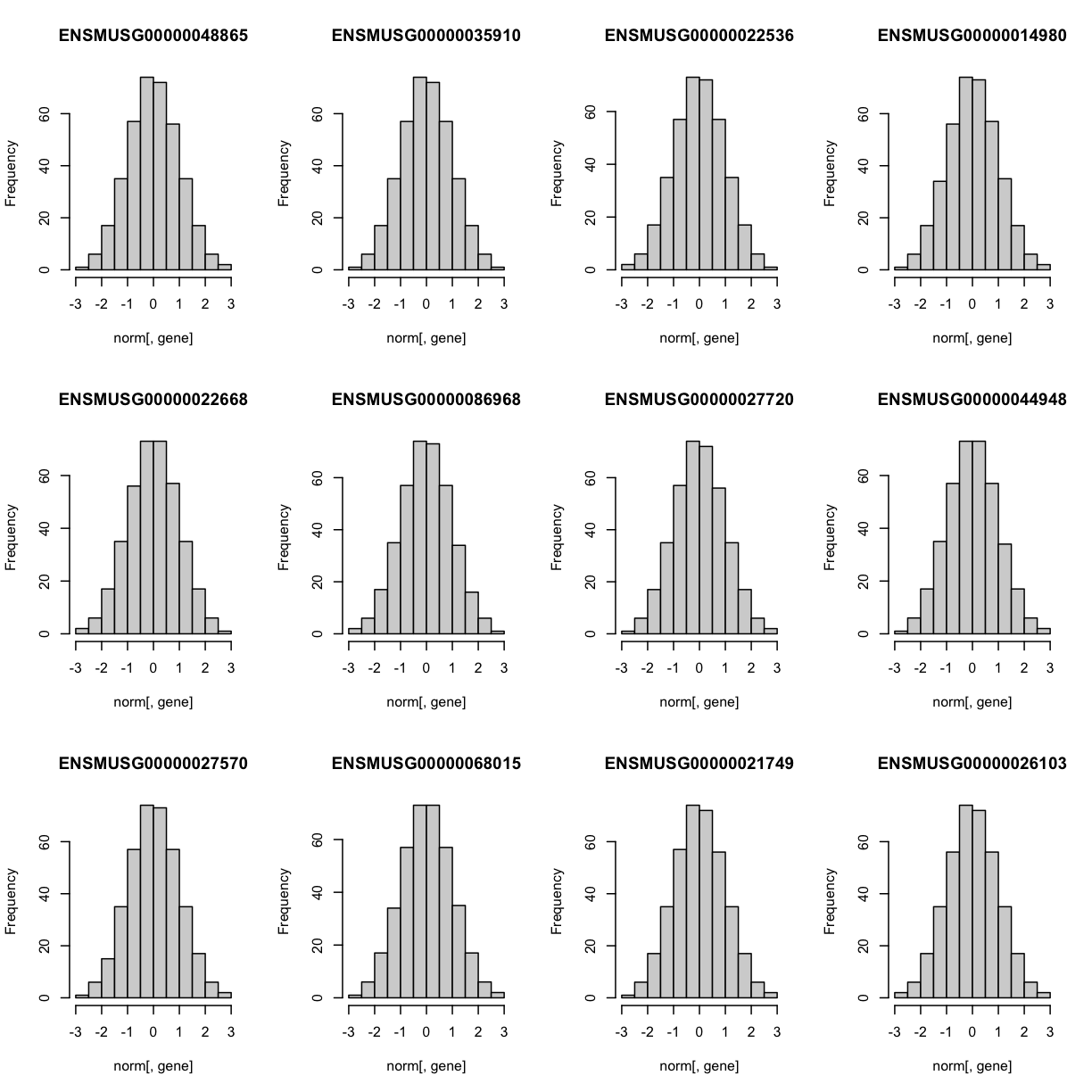
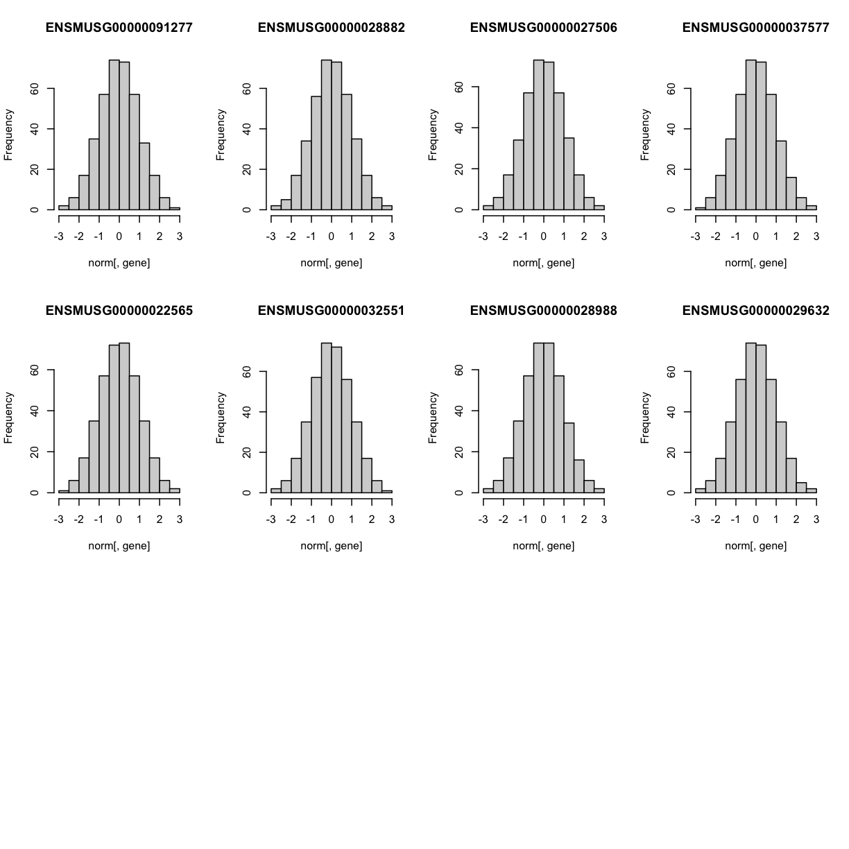 The histogram indicates that distribution of these counts are normalised (as they should be).
The Marker Map
We are using the same marker map as in the previous lesson
Genotype probabilities
We have explored this earlier in th previous lesson. But, as a reminder, we have already calculated genotype probabilities which we loaded above called probs. This contains the 8 state genotype probabilities using the 69k grid map of the same 500 DO mice that also have clinical phenotypes.
Kinship Matrix
We have explored the kinship matrix in the previous lesson. It has already been calculated and loaded in above.
Covariates
Now let’s add the necessary covariates. For these 50 gene expression data, let’s see which covariates are significant.
###merging covariate data and expression data to test for sex, wave and diet_days.

cov.counts <- merge(covar, norm[,genes], by=c("row.names"), sort=F)

#testing covairates on expression data

tmp = cov.counts %>%
        dplyr::select(mouse, sex, DOwave, diet_days, names(cov.counts[,genes])) %>%
        gather(expression, value, -mouse, -sex, -DOwave, -diet_days) %>%
        group_by(expression) %>%
        nest()
mod_fxn = function(df) {
  lm(value ~ sex + DOwave + diet_days, data = df)
}
tmp = tmp %>%
  mutate(model = map(data, mod_fxn)) %>%
  mutate(summ = map(model, tidy)) %>%
  unnest(summ)
#  kable(tmp, caption = "Effects of Sex, Wave & Diet Days on Expression")

tmp
# A tibble: 200 × 8
# Groups: expression [50]
expression data model term estimate std.e…¹ stati…² p.value
<chr> <list> <list> <chr> <dbl> <dbl> <dbl> <dbl>
1 ENSMUSG00000048865 <tibble> <lm> (Interce… 0.628 0.620 1.01 0.311
2 ENSMUSG00000048865 <tibble> <lm> sexM -0.178 0.101 -1.76 0.0791
3 ENSMUSG00000048865 <tibble> <lm> DOwave -0.0464 0.0454 -1.02 0.308
4 ENSMUSG00000048865 <tibble> <lm> diet_days -0.00327 0.00474 -0.690 0.491
5 ENSMUSG00000035910 <tibble> <lm> (Interce… 0.227 0.616 0.369 0.713
6 ENSMUSG00000035910 <tibble> <lm> sexM 0.167 0.100 1.66 0.0972
7 ENSMUSG00000035910 <tibble> <lm> DOwave -0.0359 0.0451 -0.795 0.427
8 ENSMUSG00000035910 <tibble> <lm> diet_days -0.00172 0.00470 -0.365 0.715
9 ENSMUSG00000022536 <tibble> <lm> (Interce… -0.188 0.512 -0.368 0.713
10 ENSMUSG00000022536 <tibble> <lm> sexM -0.0204 0.0834 -0.245 0.806
# … with 190 more rows, and abbreviated variable names ¹std.error, ²statistic
tmp %>%
  filter(term != "(Intercept)") %>%
  mutate(neg.log.p = -log10(p.value)) %>%
  ggplot(aes(term, neg.log.p)) +
    geom_point() +
    facet_wrap(~expression, ncol=10) +
    labs(title = "Significance of Sex, Wave & Diet Days on Expression") +
    theme(axis.text.x = element_text(angle = 90, hjust = 1, vjust = 0.5)) +
rm(tmp)
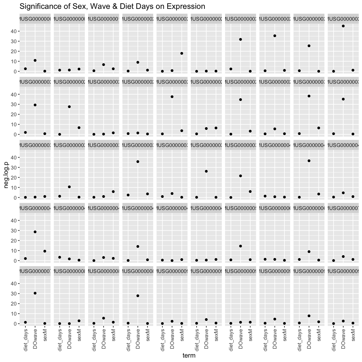
We can see that DOwave is the most significant. However, given that a few are influenced by sex and diet_days, we will have to correct for those as well.
# convert sex and DO wave (batch) to factors
pheno_clin$sex = factor(pheno_clin$sex)
pheno_clin$DOwave = factor(pheno_clin$DOwave)
pheno_clin$diet_days = factor(pheno_clin$DOwave)

covar = model.matrix(~sex + DOwave + diet_days, data = pheno_clin)
Performing a genome scan
Now lets perform the genome scan! We are also going to save our qtl results in an Rdata file to be used in further lessons.
QTL Scans
qtl.file = "../results/gene.norm_qtl_cis.trans.Rdata"

if(file.exists(qtl.file)) {
  load(qtl.file)
  } else {
    qtl = scan1(genoprobs = probs,
                pheno = norm[,genes, drop = FALSE],
                kinship = K,
                addcovar = covar,
                cores = 2)
    save(qtl, file = qtl.file)
    }
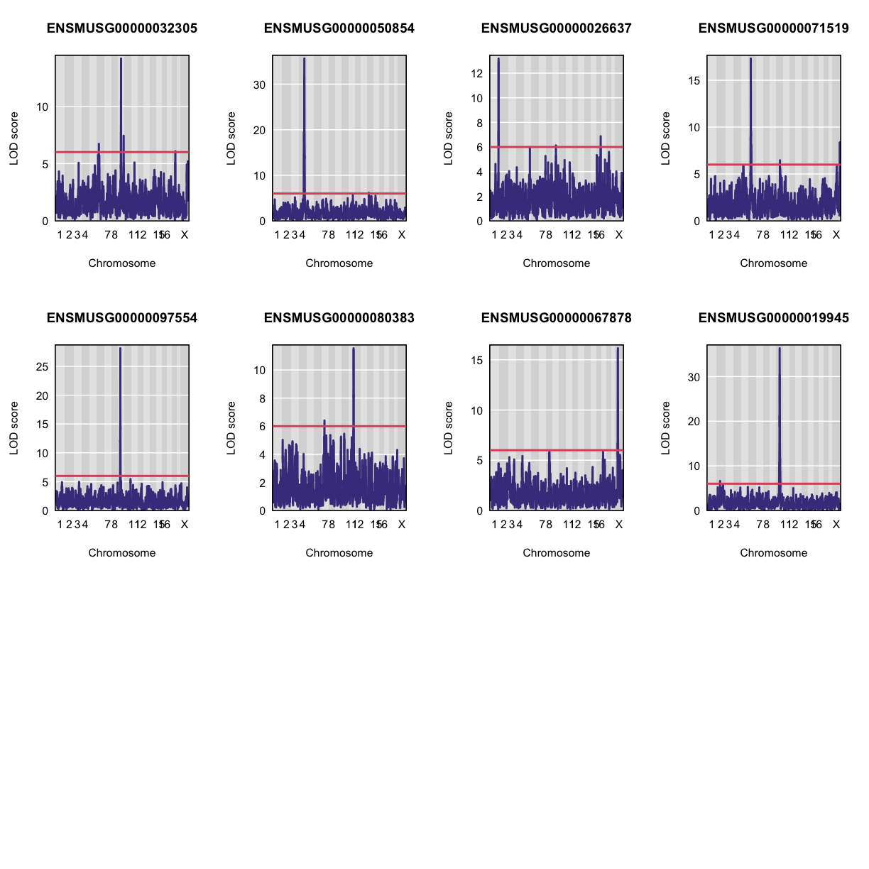
QTL plots
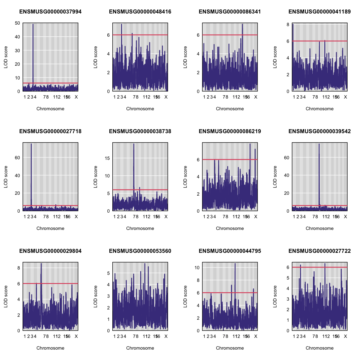
Let’s plot the first 20 gene expression phenotypes. If you would like to plot all 50, change for(i in 1:20) in the code below to for(i in 1:ncol(qtl)).
par(mfrow=c(3,4))
for(i in 1:20) {
  plot_scan1(x = qtl,
             map = map,
             lodcolumn = i,
             main = colnames(qtl)[i])
  abline(h = 6, col = 2, lwd = 2)
  }
QTL Peaks
We are also going to save our peak results so we can use these again else where. First, lets get out peaks with a LOD score greater than 6.
lod_threshold = 6
peaks = find_peaks(scan1_output = qtl,
                   map = map,
                   threshold = lod_threshold,
                   peakdrop = 4,
                   prob = 0.95)
We will save these peaks into a csv file.
kable(peaks %>%
        dplyr::select(-lodindex) %>%
        arrange(chr, pos), caption = "Expression QTL (eQTL) Peaks with LOD >= 6")

write_csv(peaks, "../results/gene.norm_qtl_peaks_cis.trans.csv")
Table: Phenotype QTL Peaks with LOD >= 6
| lodcolumn | chr | pos | lod | ci_lo | ci_hi |
|---|---|---|---|---|---|
| ENSMUSG00000033389 | 1 | 24.116007 | 6.296328 | 18.001823 | 32.48454 |
| ENSMUSG00000041189 | 1 | 38.681019 | 8.009293 | 37.690607 | 38.99625 |
| ENSMUSG00000015112 | 1 | 74.157715 | 6.390019 | 73.792993 | 190.01604 |
| ENSMUSG00000058420 | 1 | 190.002808 | 6.531293 | 135.481336 | 191.89737 |
| ENSMUSG00000026637 | 1 | 192.137668 | 13.183821 | 191.655992 | 192.51205 |
| ENSMUSG00000019945 | 2 | 72.077418 | 6.609965 | 17.713445 | 169.28966 |
| ENSMUSG00000081046 | 2 | 129.184651 | 6.497957 | 12.915206 | 135.45041 |
| ENSMUSG00000097283 | 2 | 153.419672 | 8.793228 | 150.991127 | 153.83765 |
| ENSMUSG00000027487 | 2 | 156.136279 | 6.608979 | 154.085478 | 156.75363 |
| ENSMUSG00000027487 | 2 | 161.576254 | 7.091103 | 161.309135 | 162.89119 |
| ENSMUSG00000054455 | 2 | 165.445995 | 8.888555 | 163.582672 | 166.47560 |
| ENSMUSG00000097283 | 2 | 178.833418 | 30.515193 | 176.416737 | 178.90319 |
| ENSMUSG00000027718 | 3 | 33.606276 | 31.217791 | 32.304940 | 33.65661 |
| ENSMUSG00000027718 | 3 | 37.165286 | 75.126515 | 36.852209 | 37.32921 |
| ENSMUSG00000027722 | 3 | 37.374870 | 6.214390 | 34.262328 | 114.46680 |
| ENSMUSG00000048416 | 3 | 67.791179 | 7.134414 | 66.785770 | 73.56933 |
| ENSMUSG00000000340 | 3 | 114.948141 | 9.484962 | 111.607392 | 114.97076 |
| ENSMUSG00000037994 | 3 | 135.232817 | 49.079161 | 135.232817 | 135.23282 |
| ENSMUSG00000021127 | 4 | 3.798433 | 6.132635 | 3.000000 | 149.94046 |
| ENSMUSG00000070980 | 4 | 54.766817 | 11.218926 | 54.527023 | 55.60324 |
| ENSMUSG00000096177 | 4 | 65.427487 | 8.792047 | 63.528309 | 78.76958 |
| ENSMUSG00000033389 | 4 | 111.238045 | 6.214717 | 109.522381 | 116.12848 |
| ENSMUSG00000050854 | 4 | 118.471245 | 35.618326 | 118.397472 | 118.54342 |
| ENSMUSG00000029804 | 4 | 143.211132 | 6.035045 | 138.750051 | 148.34659 |
| ENSMUSG00000029321 | 4 | 154.874097 | 6.069940 | 20.129417 | 156.21626 |
| ENSMUSG00000081046 | 5 | 98.997378 | 6.773936 | 92.854978 | 103.17849 |
| ENSMUSG00000029321 | 5 | 103.614608 | 21.562401 | 103.586587 | 105.67241 |
| ENSMUSG00000099095 | 5 | 108.046168 | 6.777903 | 102.956536 | 112.75631 |
| ENSMUSG00000032305 | 6 | 37.349577 | 6.720697 | 16.376879 | 48.92068 |
| ENSMUSG00000071519 | 6 | 41.406513 | 17.315115 | 40.920539 | 41.40651 |
| ENSMUSG00000002797 | 6 | 54.997148 | 39.222855 | 54.855033 | 55.18362 |
| ENSMUSG00000029804 | 6 | 58.488862 | 8.546978 | 40.993625 | 60.76170 |
| ENSMUSG00000089634 | 6 | 86.133168 | 11.672479 | 85.420854 | 86.55060 |
| ENSMUSG00000048416 | 6 | 125.226964 | 6.154786 | 45.277826 | 125.94593 |
| ENSMUSG00000031532 | 6 | 125.553788 | 6.312708 | 63.210018 | 126.65001 |
| ENSMUSG00000070980 | 6 | 127.078807 | 6.130341 | 126.722486 | 135.05159 |
| ENSMUSG00000080968 | 6 | 133.867522 | 6.004287 | 129.390996 | 139.21454 |
| ENSMUSG00000015112 | 6 | 134.185817 | 6.123813 | 129.110159 | 135.65721 |
| ENSMUSG00000070980 | 6 | 145.839910 | 6.202777 | 145.391545 | 146.31853 |
| ENSMUSG00000025557 | 7 | 36.613646 | 6.506206 | 35.767556 | 133.15669 |
| ENSMUSG00000038738 | 7 | 44.445619 | 19.010804 | 43.844466 | 44.86733 |
| ENSMUSG00000080383 | 7 | 57.912994 | 6.407887 | 50.696529 | 101.62734 |
| ENSMUSG00000058420 | 7 | 118.237771 | 29.916509 | 117.782005 | 118.45922 |
| ENSMUSG00000021676 | 8 | 22.086620 | 6.149473 | 18.457359 | 115.32557 |
| ENSMUSG00000031532 | 8 | 33.827024 | 17.787609 | 33.095603 | 34.20777 |
| ENSMUSG00000002797 | 8 | 95.702894 | 6.560175 | 94.937120 | 103.87985 |
| ENSMUSG00000049307 | 9 | 14.764262 | 117.447471 | 14.703558 | 14.84658 |
| ENSMUSG00000054455 | 9 | 27.198455 | 7.336424 | 20.908490 | 110.55064 |
| ENSMUSG00000097554 | 9 | 41.186050 | 28.140130 | 40.780764 | 41.20384 |
| ENSMUSG00000039542 | 9 | 49.615275 | 75.098477 | 49.494008 | 50.10869 |
| ENSMUSG00000038738 | 9 | 50.108691 | 6.657000 | 49.051211 | 78.22393 |
| ENSMUSG00000038086 | 9 | 51.898259 | 9.842327 | 51.472947 | 52.50449 |
| ENSMUSG00000032305 | 9 | 57.362395 | 14.166389 | 57.359763 | 57.96257 |
| ENSMUSG00000039542 | 9 | 58.357965 | 24.965759 | 58.264792 | 58.51857 |
| ENSMUSG00000026637 | 9 | 66.202095 | 6.128876 | 61.127900 | 118.85930 |
| ENSMUSG00000039542 | 9 | 107.647626 | 6.709880 | 103.046146 | 108.28455 |
| ENSMUSG00000032305 | 9 | 117.664006 | 7.429687 | 116.937976 | 118.80569 |
| ENSMUSG00000044795 | 10 | 22.909158 | 7.195228 | 21.125750 | 23.14018 |
| ENSMUSG00000019945 | 10 | 68.436555 | 36.340070 | 68.296752 | 68.55129 |
| ENSMUSG00000019945 | 10 | 68.966184 | 32.570583 | 68.966184 | 69.22692 |
| ENSMUSG00000071519 | 10 | 75.574081 | 6.462753 | 73.705382 | 83.04843 |
| ENSMUSG00000029321 | 10 | 125.591103 | 7.538025 | 125.539735 | 126.86601 |
| ENSMUSG00000080968 | 11 | 16.903986 | 6.044069 | 9.065479 | 41.96490 |
| ENSMUSG00000069910 | 11 | 34.822220 | 26.757661 | 34.701511 | 34.82222 |
| ENSMUSG00000033389 | 11 | 65.063246 | 9.777574 | 64.648612 | 68.88967 |
| ENSMUSG00000041189 | 11 | 67.078257 | 6.065475 | 64.368932 | 70.61624 |
| ENSMUSG00000044795 | 11 | 68.892129 | 10.613848 | 65.096598 | 69.41636 |
| ENSMUSG00000027722 | 11 | 73.111862 | 6.349757 | 73.005652 | 77.67011 |
| ENSMUSG00000039542 | 11 | 78.151256 | 6.402459 | 5.561303 | 105.51410 |
| ENSMUSG00000027718 | 11 | 79.152432 | 6.886785 | 70.782062 | 82.07630 |
| ENSMUSG00000051452 | 11 | 84.107102 | 10.077904 | 83.647144 | 84.68618 |
| ENSMUSG00000025557 | 11 | 98.275118 | 6.140239 | 90.223909 | 99.34041 |
| ENSMUSG00000080383 | 11 | 109.423954 | 11.546496 | 109.406840 | 111.19709 |
| ENSMUSG00000027487 | 12 | 6.347016 | 6.708630 | 5.846368 | 11.34456 |
| ENSMUSG00000033373 | 12 | 76.788953 | 32.214804 | 76.548097 | 76.88841 |
| ENSMUSG00000021127 | 12 | 83.238468 | 6.982385 | 82.129546 | 86.61000 |
| ENSMUSG00000058420 | 12 | 84.148297 | 6.072393 | 80.160035 | 117.40074 |
| ENSMUSG00000021271 | 12 | 87.166517 | 6.136045 | 56.572766 | 88.46608 |
| ENSMUSG00000049307 | 12 | 107.833410 | 6.639038 | 106.974113 | 109.52447 |
| ENSMUSG00000021271 | 12 | 110.197950 | 33.653196 | 110.180714 | 111.45223 |
| ENSMUSG00000099095 | 13 | 15.611917 | 8.154411 | 13.283182 | 18.32901 |
| ENSMUSG00000015112 | 13 | 35.457506 | 6.362942 | 34.416849 | 105.15802 |
| ENSMUSG00000027487 | 13 | 64.344624 | 9.185658 | 63.548321 | 67.69218 |
| ENSMUSG00000097283 | 13 | 65.206454 | 10.783729 | 64.841763 | 66.93469 |
| ENSMUSG00000021676 | 13 | 95.733655 | 100.243082 | 95.733655 | 95.85903 |
| ENSMUSG00000069910 | 13 | 101.786348 | 6.927969 | 101.137104 | 102.83022 |
| ENSMUSG00000050854 | 14 | 31.435803 | 6.178650 | 28.932629 | 94.70510 |
| ENSMUSG00000086341 | 14 | 48.126291 | 7.138599 | 46.678372 | 51.99293 |
| ENSMUSG00000025557 | 14 | 99.566266 | 6.659106 | 13.014489 | 101.18782 |
| ENSMUSG00000025557 | 14 | 121.571691 | 35.458616 | 121.480418 | 121.67373 |
| ENSMUSG00000022292 | 15 | 38.227976 | 7.784003 | 36.256559 | 41.45437 |
| ENSMUSG00000015112 | 15 | 58.990004 | 7.527785 | 58.658042 | 60.07672 |
| ENSMUSG00000060487 | 15 | 60.990009 | 6.909902 | 58.857152 | 67.06317 |
| ENSMUSG00000022292 | 15 | 64.643518 | 6.404510 | 62.181647 | 72.90648 |
| ENSMUSG00000024085 | 15 | 66.679768 | 7.227881 | 63.659243 | 68.92043 |
| ENSMUSG00000080968 | 15 | 100.424363 | 59.731554 | 99.800294 | 100.43483 |
| ENSMUSG00000026637 | 16 | 94.789233 | 6.874482 | 3.000000 | 94.97204 |
| ENSMUSG00000015112 | 17 | 43.242630 | 7.536525 | 34.179599 | 43.56276 |
| ENSMUSG00000024085 | 17 | 64.655048 | 55.404509 | 64.600441 | 64.72895 |
| ENSMUSG00000069910 | 17 | 69.244748 | 6.998414 | 68.506902 | 70.46603 |
| ENSMUSG00000086219 | 17 | 78.830855 | 7.823507 | 77.910515 | 80.14648 |
| ENSMUSG00000070980 | 17 | 89.875434 | 6.190791 | 78.362313 | 94.98443 |
| ENSMUSG00000032305 | 18 | 68.177134 | 6.075548 | 65.041330 | 68.20743 |
| ENSMUSG00000002797 | 19 | 38.421678 | 6.062762 | 36.662639 | 40.14056 |
| ENSMUSG00000044795 | 19 | 40.204814 | 6.610261 | 38.774165 | 40.22262 |
| ENSMUSG00000021676 | X | 12.322085 | 7.621003 | 11.895188 | 12.99006 |
| ENSMUSG00000086219 | X | 49.017962 | 7.209342 | 48.174569 | 50.20412 |
| ENSMUSG00000009079 | X | 53.140129 | 7.474459 | 51.892232 | 59.08406 |
| ENSMUSG00000067878 | X | 56.774258 | 16.144863 | 53.969865 | 56.80714 |
| ENSMUSG00000015112 | X | 150.513256 | 10.317359 | 145.335742 | 157.49709 |
| ENSMUSG00000058420 | X | 153.682008 | 7.479411 | 146.728544 | 163.71076 |
| ENSMUSG00000022292 | X | 158.566592 | 6.854800 | 155.383862 | 160.34933 |
| ENSMUSG00000071519 | X | 166.335626 | 8.361242 | 164.415283 | 167.22935 |
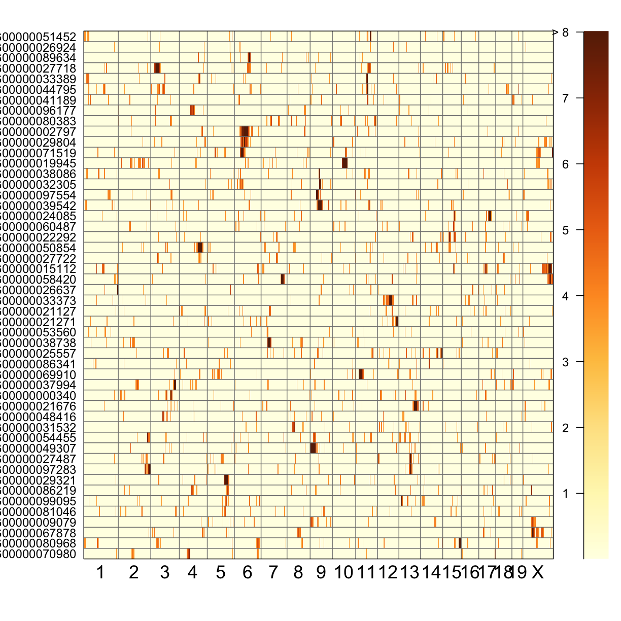
QTL Peaks Figure
qtl_heatmap(qtl = qtl, map = map, low.thr = 3.5)
Challenge
What do the qtl scans for all gene exression traits look like? Note: Don’t worry, we’ve done the qtl scans for you!!! You can read in this file,
../data/gene.norm_qtl_all.genes.Rdata, which are thescan1results for all gene expression traits.Solution
load("../data/gene.norm_qtl_all.genes.Rdata")

lod_threshold = 6
peaks = find_peaks(scan1_output = qtl,
               map = map,
               threshold = lod_threshold,
               peakdrop = 4,
               prob = 0.95)
write_csv(peaks, "../results/gene.norm_qtl_all.genes_peaks.csv")

## Heat Map
qtl_heatmap(qtl = qtl, map = map, low.thr = 3.5)
Key Points