Creating A Transcriptome Map

Overview

Teaching: 30 min
Exercises: 30 min

Questions

How do I create and interpret a transcriptome map?

Objectives

Describe a transcriptome map.

Interpret a transcriptome map.

Load Libraries

library(tidyverse)
library(qtl2)
library(qtl2convert)
library(GGally)
library(broom)
library(corrplot)
library(RColorBrewer)
library(qtl2ggplot)

source("../code/gg_transcriptome_map.R")
source("../code/qtl_heatmap.R")

Load Data

#expression data
load("../data/attie_DO500_expr.datasets.RData")

##mapping data
load("../data/attie_DO500_mapping.data.RData")

##genoprobs
probs = readRDS("../data/attie_DO500_genoprobs_v5.rds")

##phenotypes
load("../data/attie_DO500_clinical.phenotypes.RData")

expr.mrna <- norm

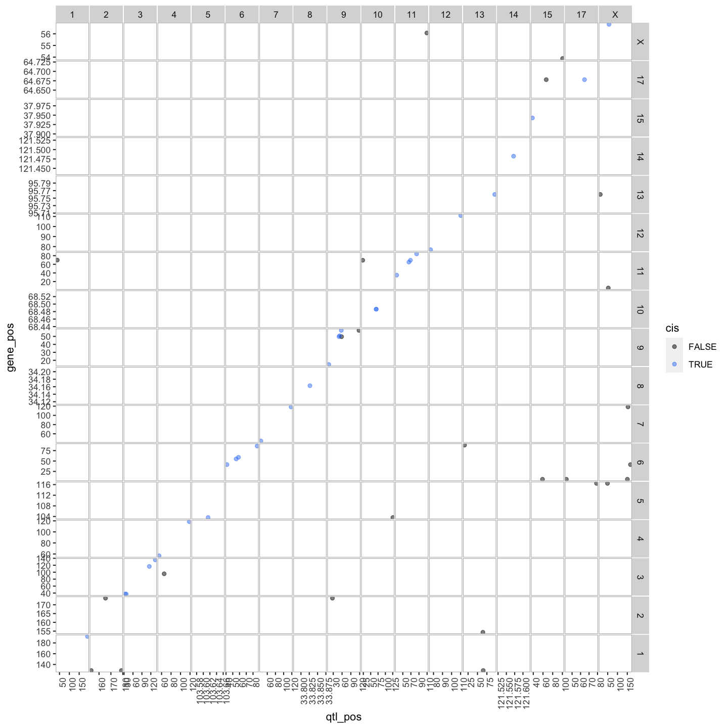
In this lesson we are going to learn how to create a transcriptome map. At transcriptome map shows the location of the eQTL peak compared its gene location, giving information about cos and trans eQTLs.

We are going to use the file that we created in the previous lesson with the lod scores greater than 6: gene.norm_qtl_peaks_cis.trans.csv.

You can load it in using the following code:

lod_summary = read.csv("../results/gene.norm_qtl_peaks_cis.trans.csv")
lod_summary$marker.id <- paste0(lod_summary$chr,
                                "_",
                                lod_summary$pos * 1000000)

ensembl = get_ensembl_genes()

snapshotDate(): 2022-04-25

loading from cache

Importing File into R ..

id    = ensembl$gene_id
chr   = seqnames(ensembl)
start = start(ensembl) * 1e-6
end   = end(ensembl)   * 1e-6
df = data.frame(ensembl = id, 
                gene_chr = chr, 
                gene_start = start, 
                gene_end = end,
                stringsAsFactors = F)
colnames(lod_summary)[colnames(lod_summary) == "lodcolumn"] = "ensembl"
colnames(lod_summary)[colnames(lod_summary) == "chr"] = "qtl_chr"
colnames(lod_summary)[colnames(lod_summary) == "pos"] = "qtl_pos"
colnames(lod_summary)[colnames(lod_summary) == "lod"] = "qtl_lod"
lod_summary = left_join(lod_summary, df, by = "ensembl")
lod_summary = mutate(lod_summary, 
                     gene_chr = factor(gene_chr, levels = c(1:19, "X")),
                     qtl_chr = factor(qtl_chr, levels = c(1:19, "X")))
rm(df)

We can summarise which eQTLs are cis or trans. Remember a cis qtl is… and trans eqtl is….

lod_summary$cis.trans <- ifelse(lod_summary$qtl_chr == lod_summary$gene_chr, "cis", "trans")
table(lod_summary$cis.trans)

  cis trans 
   47    65 

Plot Transcriptome Map

lod_summary = mutate(lod_summary, cis = (gene_chr == qtl_chr) & (abs(gene_start - qtl_pos) < 4))
out.plot = ggtmap(data = lod_summary %>% filter(qtl_lod >= 7.18), cis.points = TRUE, cis.radius = 4)

plot of chunk unnamed-chunk-2

pdf("../results/transcriptome_map_cis.trans.pdf", width = 10, height = 10)
out.plot
dev.off()

quartz_off_screen 
                2 

out.plot

plot of chunk unnamed-chunk-2

Key Points

Transcriptome maps aid in understanding gene expression regulation.

previous episode

Gene Expression QTL Analysis

next episode